Impedance calculations

Impedance of the 13cm filter

As we all know, Impedance matching is important. So we like to know, how good this matching is. Therefore we like to measure it. Using a VNA we get S-Parameters, calculating Impedance from them seems to be easy:

\[ Z_L = Z_0 \frac{1 + S_{11}}{1 - S_{11}} \]

\(Z_L = Z(f)\) means impedance depending on frequency

\(Z_0 = 50 \Omega\) is standard impedance

\(S_{11}\) is the measured S-Parameter

Python, scikit.rf and numpy module shold fit. The s-parameters we have already on file.

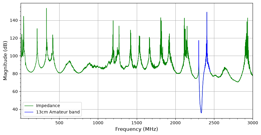
import numpy as np
from skrf import Network, Frequency
import matplotlib
import matplotlib.pyplot as plt
import os

def impedance_from_s_param(network, impedance_file="imped.s1p"):
    """calculate impedance from networks s11-parameters for every frequency
    and write impedance file as touchstone for later usage.
    """
    new_filename = impedance_file
    frq = network.f
    s11 = network.s[:,0,0]
    imp = network.subnetwork([0])
    imp.name = new_filename
    z0 = 50
    for i in range(len(frq)):
        a = s11[i].real
        b = s11[i].imag
        gamma = (abs((a**2 + b**2) ** 0.5))
        vswr = abs((1+gamma) / (1-gamma))
        zl = z0 * vswr
        imp.s[i] = zl
    imp.comments = "Impedances over Frequencies"
    imp.name = "Impedance"
    imp.write_touchstone(new_filename)
    return imp    


Z_0 = 50     # 50 Ohms
filter = Network()
filter.read_touchstone('files/13cmInterdigitalFilterFull.s2p')
filter.name = "Filter 23cm"
# show the properties from the touchstone file
S11 = filter.s11
imped = impedance_from_s_param(S11)
imped.name = "Impedance"
print("Impedance:", S11)
# lets show what we got
plt.rcParams['figure.figsize'] = [10, 5]
plt.grid(True)
plt.minorticks_on()
plt.title = filter.name
plt.xlabel("Frequency (MHz) ", fontsize=12)
plt.ylabel("Impedance (Ohm)", fontsize=12)
#
imped.plot_s_db(c='g', lw=1, label=imped.name)
regio = '2300-2450'
imped[regio].plot_s_db(c='b', lw=1, label='13cm Amateur band')
plt.show()

Impedance: 1-Port Network: 'Filter 23cm',  1.0-3000.0 MHz, 4501 pts, z0=[50.+0.j]

This looks strange, only the interesting part, resp. the 13cm amateur band, in parts shows an accaeptable impedance of \(50 \Omega\), lets zoom in.

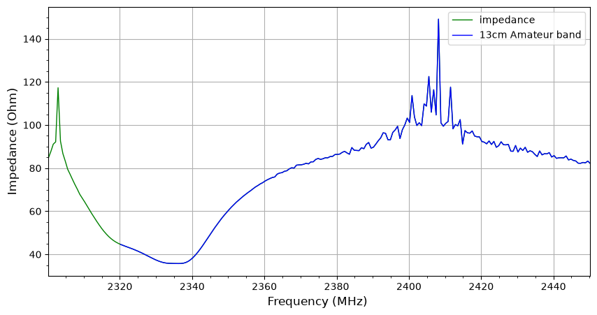
zoom = '2300-2450'
s11 = filter.s11[zoom]
s11.name = "s11"
imped = impedance_from_s_param(s11)
imped.name = "impedance"
print(s11, "(zoom range is fitted onto the available calibration points)")
plt.rcParams['figure.figsize'] = [10, 5]
plt.grid(True)
plt.minorticks_on()
plt.title = filter.name
imped.plot_s_db(c='g', lw=1, label=imped.name)
regio = '2320-2450'
imped[regio].plot_s_db(c='b', lw=1, label='13cm Amateur band')
plt.xlabel("Frequency (MHz) ", fontsize=12)
plt.ylabel("Impedance (Ohm)", fontsize=12)
plt.show()

1-Port Network: 's11',  2300.233333-2450.183333 MHz, 226 pts, z0=[50.+0.j] (zoom range is fitted onto the available calibration points)

The filter justified like this might not be usable for the full 13cm amateur band, but usually you will have some preferences about the used modes and not in need of the whole band.

Have Fun!