LibreVNA first measurement

I got a new LibreVNA, hooray!

It is a Zeenko product. Plain aluminum with some LEDs and four SMA-connectors.

Wonderful manuals are included printed on DIN A6 paper to fit in the box.

Nevertheless they are available at their github account as sources, so I can have my own pdf files and print them on my A4 paper … Beautiful typesetting and content.

It is a 2-Port VNA. Compared to professional equipment from R&S or others, it is cheap, so I wanted to buy the LibreCAL was well. Thats a very good tool in combination, I dreamed about such funtionality with my first NanoVNA already some years ago. The fiddling with SMA-connectors I see as a boring and destroying way of doing…

My first addtional investment were some SMA portsavers to protect the sensitive SMA-ports.

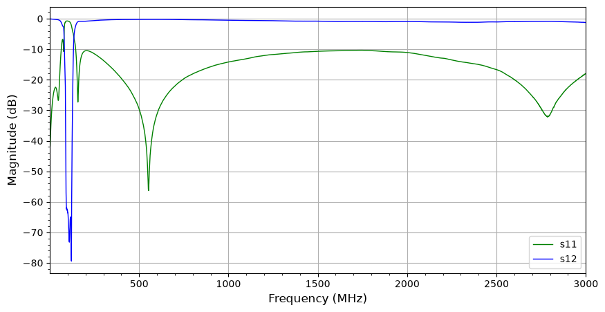
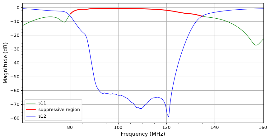
Of course I wanted to measure something immediately. An old UKW notch filter I tested first, I don’t know where it came from. Use of the filter is to suppress nearby strong broadcast radio transmitters in the the range from 87 to 108 MHz. I connected the filter to LibreVNA port 1 and port 2. From the LibreVNA-GUI app I saved a touchstone file, the used frequencies went from 1 to 3000 MHz with 4501 (max) measurement points. That would help me to zoom into the values wherever I want to.

Soon some lines of python were written …

from skrf import Network, Frequency
import matplotlib
import matplotlib.pyplot as plt
import os

filter = Network()
filter.read_touchstone('files/UKW-notch-1.s2p')
filter.name = "My ukw-notch"

# show the properties from the touchstone file
print("filter properties:", filter)

s11 = filter.s11
s11.name = "s11"
s12 = filter.s12
s12.name = "s12"
# lets show what we got
plt.rcParams['figure.figsize'] = [10, 5]
plt.grid(True)
plt.minorticks_on()
plt.title = filter.name
plt.xlabel("Frequency (MHz) ", fontsize=12)
plt.ylabel("Signal (db)", fontsize=12)

plt.title = filter.name
s11.plot_s_db(c='g', lw=1, label=s11.name)
s12.plot_s_db(c='b', lw=1, label=s12.name)
plt.show()

filter properties: 2-Port Network: 'My ukw-notch',  1.0-3000.0 MHz, 4501 pts, z0=[50.+0.j 50.+0.j]

So we see the whole band is rather plain except the small part around the 100 MHz. Lets try to zoom in.

s11 = filter.s11['60-160']
s11.name = "s11"
s12 = filter.s12['60-160']
s12.name = "s12"
plt.rcParams['figure.figsize'] = [10, 5]
plt.grid(True)
plt.minorticks_on()
plt.title = filter.name
plt.xlabel("Frequency (MHz) ", fontsize=12)
plt.ylabel("Signal (db)", fontsize=12)

plt.title = filter.name
s11.plot_s_db(c='g', lw=1, label=s11.name)
s11['80-135'].plot_s_db(c='r', lw=2, label='suppressive region')
s12.plot_s_db(c='b', lw=1, label=s12.name)
plt.show()

Thats all about my old notch filter…

Have Fun!